Getting Started With Getting Started
If you’ve been following this blog, you’ll know that I’ve been working on my Zmanim-WP plugin for WordPress for a while now.
If you haven’t, you can check out everything written so far using this link.
I've been working with coding agents and LLM integrations for a couple of years now. Whenever I start a coding-agent task, I explain the repository and take some time to settle the design choices. I move over to implementing a slice and expect the result. A simple loop for the agents and me. What is annoying, though, is that all the context is lost when I start a new session. And this started hindering my productivity quickly. There are plenty of alternatives for managing context and memory in coding agents. This article introduces the one that works the best for me and my workflow.
When we call a model, it does not carry durable state from one request to the next. Depending on how the harness fills the next context window from its own inputs coupled with the system prompt, tool results from the current session, and whatever files we as users attach, it generates the results. When I start a new conversation, it usually does not know anything about earlier sessions we had.
The modern enterprise generates and consumes unprecedented volumes of data across operational systems, customer interactions, partner ecosystems, cloud applications, IoT devices, and AI platforms. At the same time, AI systems are becoming major consumers of enterprise data, making decisions, generating content, recommending actions, and automating workflows.
Poor data quality is no longer just a reporting issue; it is also an AI issue. Inaccurate, incomplete, or poorly governed data can produce biased outcomes, regulatory violations, AI hallucinations, and flawed business decisions.
Rust Has Entered the Kernel. Now Comes the Dangerous Part.
A kernel driver does not fail politely.
It does not throw a friendly exception, generate a neat stack trace, and ask whether you would like to restart. It corrupts memory, wedges hardware, leaks secrets, freezes the compositor, and leaves engineers spelunking through logs at 2 a.m. with the emotional range of a haunted printer.
The Problem: Tracking Request Latency Without Slowing Things Down
For a cloud data warehouse, performance is not just about average query time. What often matters more is tail latency, predictability, and the ability to pinpoint where things go wrong. In a cloud-native data warehouse like Databend, a single request may pass through multiple stages: SQL planning, distributed execution, remote storage,
Raft logging, and state machine apply. Tail latency in any one of these stages can affect the query stability users actually experience.
That means we need a way to continuously track latency distributions inside the system — lightweight enough to stay off the hot path, accurate enough to be useful, and cheap enough to run everywhere. This article walks through the design of base2histogram, the lightweight histogram library we built for that purpose.
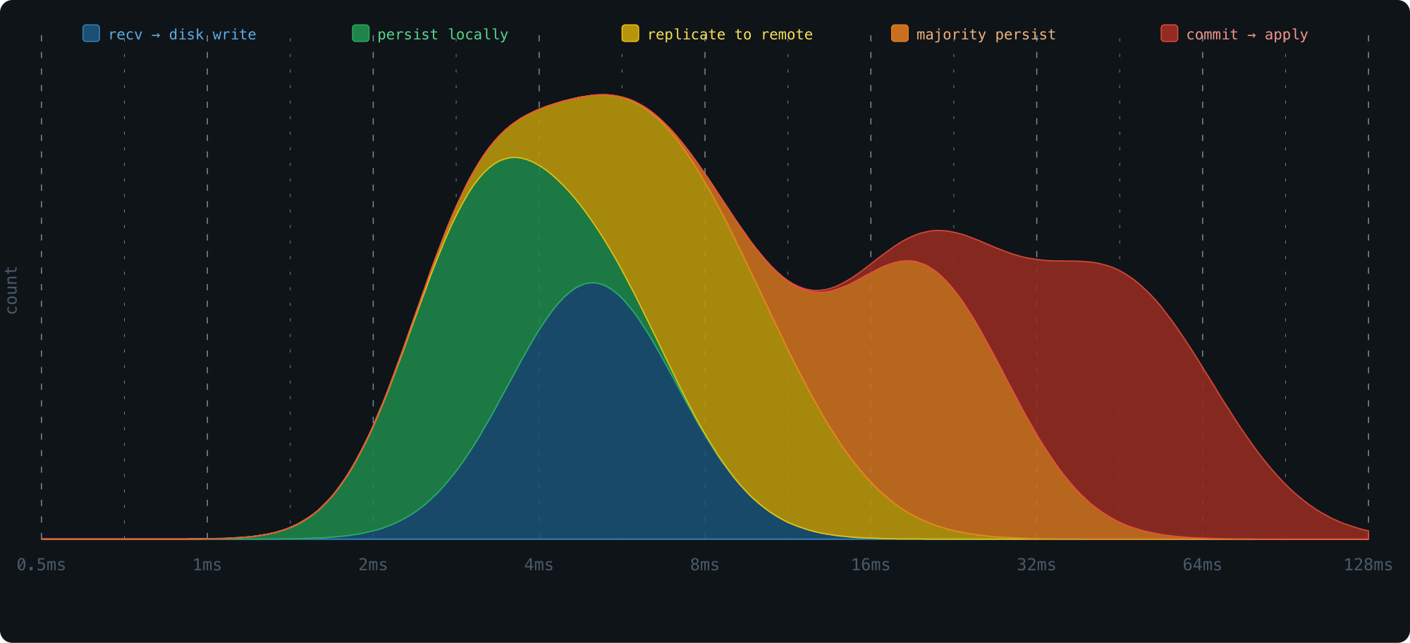
Consider the lifecycle of a single Raft log entry. It passes through several stages, each with its own latency profile:
- Received → written to storage
- Persisted to local disk
- Replicated to remote nodes
- Acknowledged by a majority quorum
- Committed → applied to the state machine
A histogram is a natural fit here: put latency on the x-axis and request count on the y-axis, and you get an immediate view of where time is being spent.
This kind of visibility helps you identify bottlenecks and fix the right part of the system.
But there is a catch: collecting metrics must not get in the way of doing actual work. The histogram needs to be:
- O(1) to record: No sorting, no rebalancing, and nothing that can stall a hot path
- Tiny in memory: A system may run hundreds or thousands of histograms at once
- Queryable for percentiles: P50, P95, P99
Let's walk through how we designed a histogram that meets all three requirements.
Recording: Getting Samples Into Buckets
Why Log-Scale Buckets
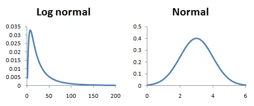
Most requests cluster around a typical latency, with a few outliers on both ends. This often produces a log-normal distribution: take the log of the latency values, and the shape becomes a classic bell curve.
The signature shape is a peak at lower values, followed by a gradual long tail to the right.
![The signature shape is a peak at lower values, followed by a gradual long tail to the right.]()
To build a histogram, we divide the x-axis into buckets and count how many samples fall into each one.
The key question is how to size those buckets.
Equal-width buckets work well for a normal distribution, but latency is often log-normal. The data only looks roughly uniform on a logarithmic scale, so the buckets should grow on a log scale, not a linear one.
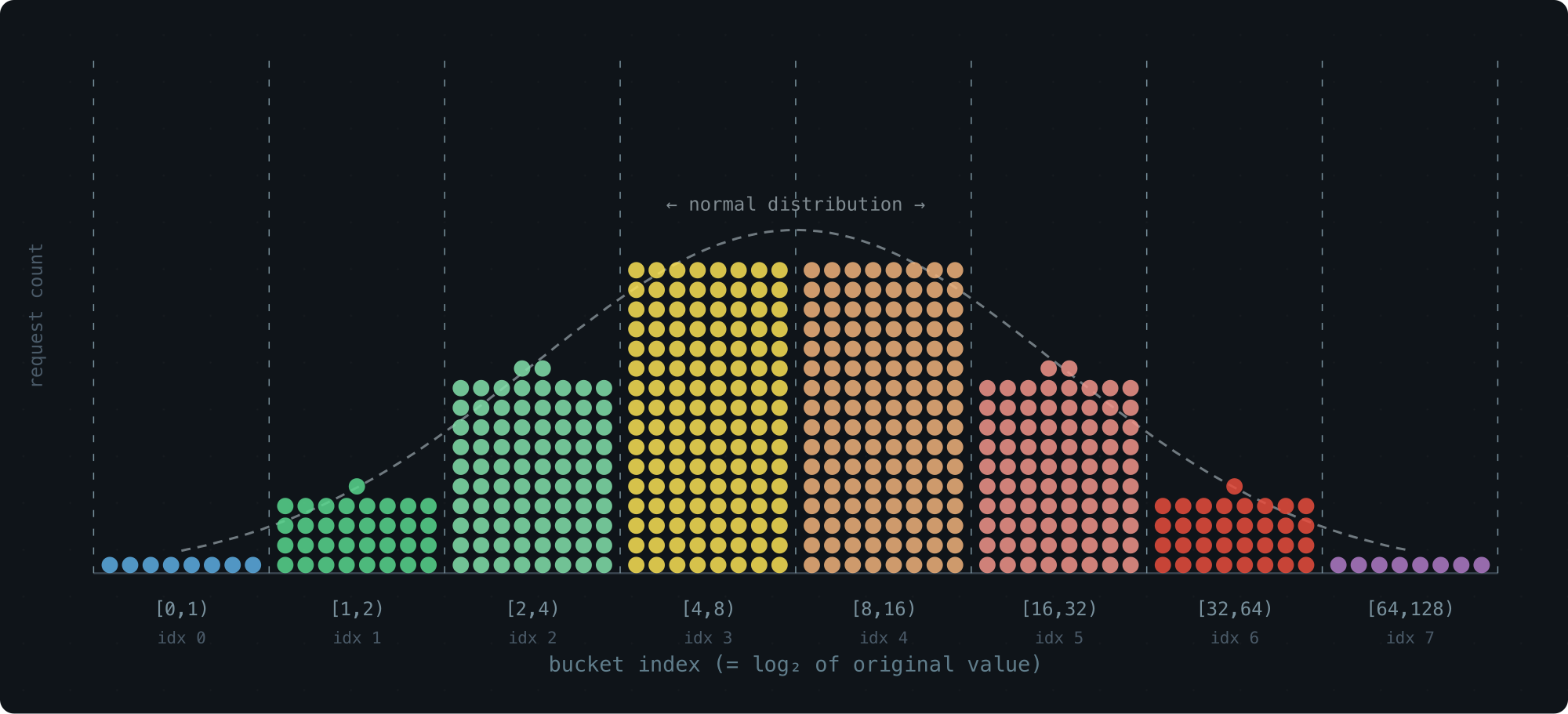
The simplest version is to make each bucket twice as wide as the previous one:[0,1), [1,2), [2,4), [4,8), [8,16), ...Why powers of 2? Because multiplying by 2 is cheap on a CPU, and mapping a value to its bucket takes a single leading-zero-count instruction.
If we simulate a log-normal workload and plot bucket counts with the bucket index on the x-axis — effectively applying a log transform — the result is a clean bell curve:
This is great for storage: 65 buckets cover the entire u64range.
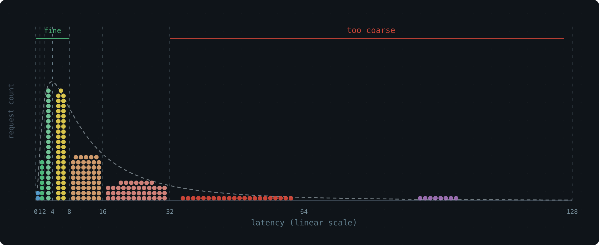
But the resolution is poor. The last bucket spans half of all possible values, so everything that lands there becomes a blur.
A Tempting Fix We Passed On
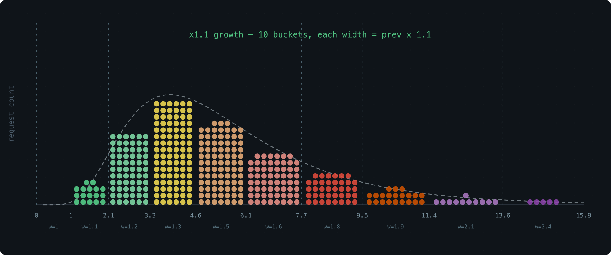
An obvious improvement is to use a smaller growth factor, such as 1.1× instead of 2×. That gives us more buckets and finer resolution:
The problem is cost. Finding the right bucket for a value l means solving for the smallest x where 1 + 1.1 + 1.1^2 + ... + 1.1^x >= l, which requires floating-point logarithms. That is real overhead on a hot path.
We wanted to stay in the world of integers and bit operations.
The Trick: Float-Like Encoding
Here is the idea that makes the design work: keep bucket sizes roughly exponential, but encode each bucket using a fixed number of bits — a parameter we call WIDTH.
Think of a bucket's lower bound as a tiny floating-point number.
The MSB position gives the exponent, which tells us which bucket group the value belongs to. The next few bits give the offset within that group.
With WIDTH=3, the default configuration, a bucket boundary looks like this in binary:
00..00 1 xx 00..00
       |
       MSB
<- significant
The leading 1selects the group. The two bits that follow select the bucket within the group.
Here is what the first few groups look like. Each bucket is fully described by just 3 bits:
WIDTH = 3:

range     bucket index        bucket size
[0, 1)     0  0b0 ..... 000    1
[1, 2)     1  0b0 ..... 001    1
[2, 3)     2  0b0 ..... 010    1
[3, 4)     3  0b0 ..... 011    1

[4, 5)     4  0b0 ..... 100    1
[5, 6)     5  0b0 ..... 101    1
[6, 7)     6  0b0 ..... 110    1
[7, 8)     7  0b0 ..... 111    1

[8, 10)    8  0b0 .... 1000    2
[10, 12)   9  0b0 .... 1010    2
[12, 14)  10  0b0 .... 1100    2
[14, 16)  11  0b0 .... 1110    2

[16, 20)  12  0b0 ... 10000    4
[20, 24)  13  0b0 ... 10100    4
[24, 28)  14  0b0 ... 11000    4
[28, 32)  15  0b0 ... 11100    4

[32, 40)  16  0b0 .. 100000    8
[40, 48)  17  0b0 .. 101000    8
[48, 56)  18  0b0 .. 110000    8
[56, 64)  19  0b0 .. 111000    8




Comments
Post a Comment